
The vision layer gives you 21 points floating in a normalized coordinate space that has no physical units and a faked depth axis. The mechanical layer gives you fifteen revolute joints, each with a lower and upper bound in radians that came out of a CAD mate.
Nothing connects them. Building that connection is the actual work of this project, and it happens in about forty lines of Python.
flowchart LR
    A["21 landmarks
(x, y, z) normalized"] --> B["Triplet selection
15 × (p₁, p₂, p₃)"]
    B --> C["Two vectors per joint
v₁ = p₁ − p₂ · v₂ = p₃ − p₂"]
    C --> D["Dot product → arccos
θ in radians"]
    D --> E["Normalize
flexion ∈ [0, 1]"]
    E --> F["Lerp onto URDF limits
θ_urdf"]
    F --> G["JointState
names + positions"]
Step 1 — pick three points #
To measure a joint you need the joint itself and the two bones meeting at it. In landmark terms: the vertex, plus its two neighbours.
For the index finger’s PIP joint (landmark 6):
- \(P_1 = \) landmark 5, the index MCP
- \(P_2 = \) landmark 6, the index PIP — the vertex
- \(P_3 = \) landmark 7, the index DIP
Fifteen such triplets cover five digits × three joints:
triplets = [
    (0, 1, 2),   (1, 2, 3),   (2, 3, 4),      # thumb
    (0, 5, 6),   (5, 6, 7),   (6, 7, 8),      # index
    (0, 9, 10),  (9, 10, 11), (10, 11, 12),   # middle
    (0, 13, 14), (13, 14, 15),(14, 15, 16),   # ring
    (0, 17, 18), (17, 18, 19),(18, 19, 20),   # pinky
]
Look at the first entry of each group: landmark 0, the wrist. MediaPipe places no landmark at the base of each metacarpal, so for the MCP joints the wrist stands in for the metacarpal bone.
That approximation has consequences. The wrist→MCP vector is not the metacarpal’s true axis, so MCP angles are the least anatomically faithful of the three joint types — which is precisely why their URDF limits are the narrowest in the model, and why MCP is where mapping errors show up first.
Step 2 — two vectors and a dot product #
Build both vectors radiating outward from the vertex, which shifts the local origin onto the joint being measured:
$$\vec{v}_1 = P_1 - P_2 \qquad \vec{v}_2 = P_3 - P_2$$The algebraic dot product relates to the geometric angle between them by
$$\vec{v}_1 \cdot \vec{v}_2 = \lVert\vec{v}_1\rVert \, \lVert\vec{v}_2\rVert \cos(\theta)$$which rearranges to
$$\cos(\theta) = \frac{\vec{v}_1 \cdot \vec{v}_2}{\lVert\vec{v}_1\rVert \, \lVert\vec{v}_2\rVert}$$That normalization by both magnitudes is what makes the whole approach immune to MediaPipe’s faked \(z\) axis and its lack of units. Divide out both lengths and only direction survives — so it does not matter that the coordinate system has no physical scale, or that depth is compressed relative to the image plane, as long as it is compressed consistently.
Step 3 — two floating-point traps #
The line that computes \(\arccos\) is where a naive implementation crashes, and it crashes in two distinct ways.
Division by zero. MediaPipe occasionally emits two identical landmark coordinates. The bone
length is then zero, the division yields NaN, and the NaN propagates silently through the entire
message into RViz, where the model vanishes.
Domain error. \(\arccos\) is defined only on \([-1, 1]\). Floating-point arithmetic routinely
produces 1.0000000002 for two nearly-parallel vectors, and np.arccos raises on it.
Both guards are unremarkable and both are mandatory:
norm1, norm2 = np.linalg.norm(v1), np.linalg.norm(v2)
if norm1 < 1e-6 or norm2 < 1e-6:
    angles.append(0.0)
else:
    cosang = np.clip(np.dot(v1, v2) / (norm1 * norm2), -1.0, 1.0)
    angles.append(float(np.arccos(cosang)))
The output is an interior angle in radians. Intuition for the range:
| Hand pose | Interior angle | Radians |
|---|---|---|
| Finger fully straight | ≈ 177° | ≈ 3.10 |
| Finger curled into a fist | ≈ 90° | ≈ 1.60 |
A straight finger measures near \(\pi\) rather than exactly \(\pi\) because the bones are never perfectly collinear — real anatomy has a slight bias even at full extension.
Step 4 — normalize into flexion #
The raw angle is a biometric measurement. The URDF wants a mechanical one. The bridge is a dimensionless ratio:
$$\text{flexion} = \frac{\text{RAW\_STRAIGHT} - \theta}{\text{RAW\_STRAIGHT} - \text{RAW\_CURLED}}$$with the two constants read straight off the table above:
RAW_STRAIGHT_ANGLE = 3.10   # ~177°, open hand
RAW_CURLED_ANGLE   = 1.60   # ~90°,  bent finger
These are calibration constants, not derived ones. They define which slice of human motion gets stretched across the mechanism’s full travel. They are the first thing to adjust when the whole hand under- or over-flexes, and they are per-installation: a different person’s hand, or a camera at a different angle, shifts the usable window.
The clip is not optional either:
flexion = float(np.clip(flexion, 0.0, 1.0))Hyperextend a finger past the straight baseline and the numerator goes negative; a tracking glitch can push it past 1. Without the clip, either case drives the joint outside its limits.
Step 5 — interpolate onto the real mechanism #
With flexion in \([0, 1]\), the final step is a linear interpolation onto that specific joint’s mechanical range:
$$\theta_{\text{urdf}} = \theta_{\text{open}} + \text{flexion} \times (\theta_{\text{closed}} - \theta_{\text{open}})$$Each joint’s endpoints come from the URDF — literally, read at node startup rather than copied into Python:
def load_urdf_limits(urdf_path):
    root = ET.parse(urdf_path).getroot()
    limits = {}
    for joint in root.findall('joint'):
        limit = joint.find('limit')
        if limit is None:
            continue
        limits[joint.get('name')] = (float(limit.get('lower')),
                                     float(limit.get('upper')))
    return limits
So the fifteen-row JOINT_MAPPING table holds no angles at all. It holds the one fact the URDF
cannot express:
JOINT_MAPPING = [
    # (urdf joint name, mediapipe index, which limit is the open hand)
    ('thumb_mcp',   0, 'lower'),
    ('index_mcp',   3, 'upper'),
    ('middle_pip',  7, 'lower'),
    ...
]
Why the open end differs between rows #
thumb_mcp opens at its lower limit and closes at its upper. index_mcp does the reverse.
This is not inconsistency. Each mate in Onshape was constructed with its own axis orientation, so
“positive rotation” means a different physical direction per joint. Nothing in the URDF records
which direction is anatomically “open” — a <limit> is just two numbers. So that one bit per joint
has to live in code, and the interpolation handles the rest.
Normalizing every joint to a common convention would mean editing the CAD or post-processing the URDF, and would gain nothing. Encoding reality beats fighting it.
The earlier version of this table stored the angles too, copied out of the URDF by hand. That is what the next section is about.
The URDF side of the contract #
The other half of the contract is the robot description itself: a tree of rigid bodies connected by
constrained joints, generated by onshape-to-robot from the CAD.
base_link is a virtual origin with a near-zero mass (1e-09) that anchors the robot in world
space, connected by a fixed joint to part_1, the palm. Every finger hangs off the palm.
That near-zero mass is not quite free, incidentally. KDL — which robot_state_publisher uses to
build the kinematic chain — wants the root link to carry no <inertial> block at all, and logs a
warning at every startup because this one does. Harmless in practice, since nothing integrates the
root’s dynamics, but it is a real objection rather than a clean bill of health.
Each link carries three blocks:
<inertial>— mass, centre of mass and the rotational inertia matrix. RViz ignores these entirely; a physics engine cannot function without them.<visual>— which STL to draw, with its material and offset.<collision>— the boundary geometry for contact. In this auto-generated file it points at the same STLs as the visual, which is correct but expensive.
Each joint is type="revolute" with three things that matter:
<joint name="index_pip" type="revolute">
  <origin xyz="..." rpy="..."/>
  <axis xyz="0 0 1"/>
  <limit effort="10" velocity="10" lower="-1.5708" upper="2e-11"/>
</joint>
<origin> places the hinge on the parent link, <axis> says which local vector it rotates about,
and <limit> sets the mechanical bounds that JOINT_MAPPING transcribes.
Every joint in this export rotates about local Z. That is the ROS convention, and it held here — but it is worth verifying after every re-export, because the failure mode is unforgettable: fingers that bend sideways, or a digit that inverts through the palm. Nothing warns you. The transform maths is perfectly valid; it is simply describing the wrong hinge.
The naming, including twinky
#
| Digit | Joints | Links |
|---|---|---|
| Pinky | twinky_mcp twinky_pip twinky_dip |
part_2 → part_4 |
| Ring | ring_mcp ring_pip ring_dip |
part_2_2 → part_4_2 |
| Middle | middle_mcp middle_pip middle_dip |
part_2_3 → part_4_3 |
| Index | index_mcp index_pip index_dip |
part_2_4 → part_4_4 |
| Thumb | thumb_mcp thumb_pip thumb_dip |
part_5 → part_7 |
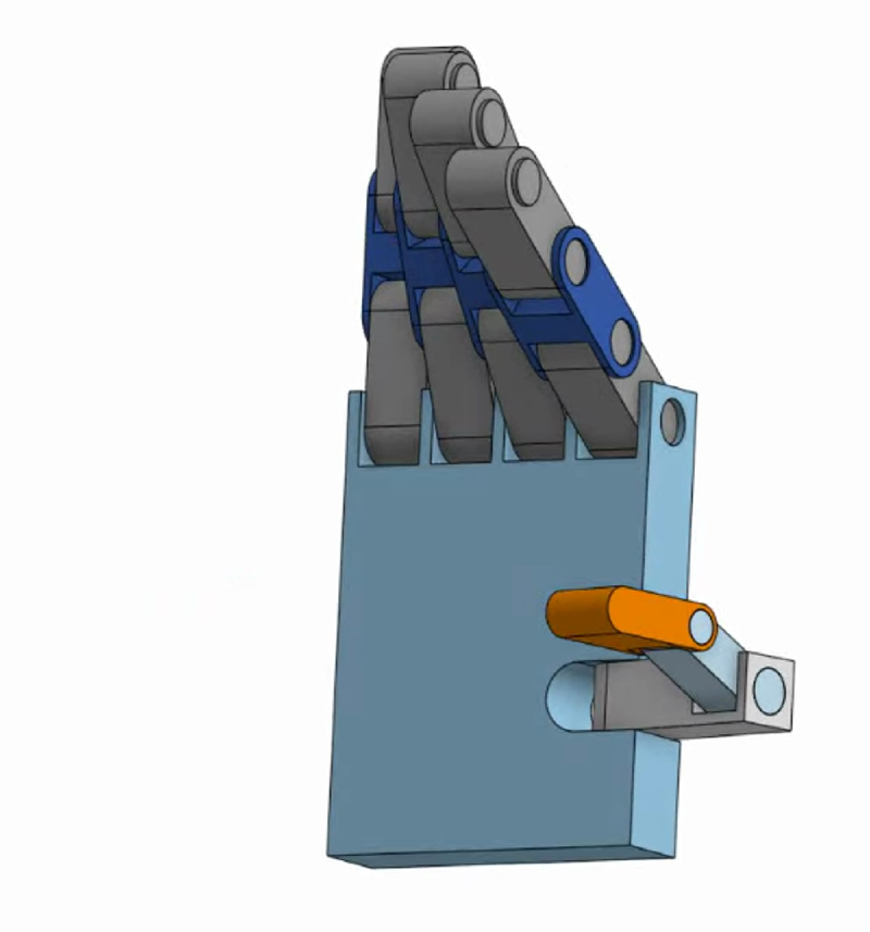
twinky is a legacy name for the pinky that survived in the Onshape mate tree. The exporter takes
the mate name, strips a dof_ prefix and uses the remainder as the joint name — so the CAD mate
dof_twinky_mcp becomes the URDF joint twinky_mcp. Because JointState matches joints by exact
string, it propagated into the Python too. Part 5 covers why it was left
alone.
A note on the abbreviations: MCP is the base knuckle (metacarpophalangeal), PIP the middle joint (proximal interphalangeal), DIP the one nearest the tip (distal interphalangeal). The thumb anatomically has a CMC and an IP rather than an MCP/PIP/DIP set, but this mechanism uses the same three-suffix scheme for all five digits — internally consistent, anatomically approximate.
Packaging it for ROS #
The mapped values are packed into a standard message with names and positions in parallel arrays:
rviz_msg = JointState()
rviz_msg.header.stamp = self.get_clock().now().to_msg()
rviz_msg.name = urdf_names
rviz_msg.position = urdf_angles
self.rviz_publisher.publish(rviz_msg)
robot_state_publisher receives this, matches each name against the URDF tree, computes forward
kinematics, and emits the resulting transforms on /tf. RViz draws whatever /tf says.
The name matching is where silent failures live. If a JointState entry names a joint that
does not exist in the URDF, robot_state_publisher does not warn — it drops it. A finger that
refuses to move while the other four work perfectly is almost always a typo, not a maths error.
The row that was wrong #
Fourteen of the fifteen rows transcribed their joint’s limits exactly. ring_mcp did not:
| Source | Open | Closed |
|---|---|---|
JOINT_MAPPING (before) |
0.000 |
-1.571 |
<limit> in the URDF |
0.39671 |
-1.17409 |
Neither endpoint matched. At full curl the node commanded −1.571 rad into a joint whose mechanical lower bound is −1.174 rad — roughly 23° past its stop.
The cause was chronological. ring_mcp originally exported with the same generic ±1.5708 bounds as
the other fingers, and the mapping was written against those. The CAD later gained a real limit for
that mate, the URDF was re-exported, and the Python table was not updated.
Nothing caught it. robot_state_publisher does not enforce URDF limits; it applies whatever
transform it is handed. RViz showed no error and no obviously broken geometry — just a ring knuckle
bending slightly further than the mechanism physically could. It would have become a hard failure
the moment this drove a physics engine or a real servo.
The row was corrected to ('ring_mcp', 9, 0.397, -1.174). But a corrected constant is a patch, not
a fix — it repairs the instance and leaves the mechanism that produced it untouched. The real
problem was a contract duplicated across two files, a URDF and a Python table, with nothing to
detect divergence.
So the limits moved. They are now parsed from the URDF at startup and exist in exactly one place,
which is why the table above holds 'lower' and 'upper' rather than numbers. Three failure modes
that used to be silent are now loud:
| Situation | Before | Now |
|---|---|---|
| URDF limit edited, Python not updated | Silent divergence | Impossible — one source |
| Joint renamed by a re-export | That finger silently freezes | RuntimeError at startup, naming the joint |
| URDF gains a joint with no mapping row | Silently never moves | Warning at startup |
The same duplicated-contract shape still sits elsewhere in the project: the hand_msgs package
exists in two copies, and a field added to one and not the other produces a subscriber that
silently never fires. Worth knowing where your second copies are.
What you should take away #
- Normalizing by both vector magnitudes is what makes a fake, unitless \(z\) axis usable.
- Clip everything. Zero-length bones and out-of-domain cosines are routine, not edge cases.
- The calibration window is per-installation, and it is the right knob for global flexion problems.
- Duplicated contracts drift. If a number lives in two files, something must check they agree — and a corrected constant is a patch, not a fix.
Next: what happens to those joint states once they leave the node.